Carrier Frequency Offset in Single Carrier and OFDM Systems

Carrier Frequency Offset (CFO) is one of the most common impairments found in a communication system. As the name suggests, it is due to the mismatch between the carrier frequencies used by the transmitter and the receiver. The effects produced by CFO on single carrier and OFDM systems is very different. To illustrate this, a simple simulation of a 64-QAM based single carrier and OFDM system using CommPy is shown below.

from numpy import real, imag, arange
from numpy.fft import fft, ifft
from numpy.random import randint
from commpy.modulation import QAMModem
from commpy.impairments import add_frequency_offset
import matplotlib.pyplot as plt

# System Parameters 
# Sampling Frequency (Hz)
Fs = 15.36e6 
# Frequency Offset (Hz)
delta_f = 500
# FFT Size for OFDM 
N = 1024

# Generate message bits
msg_bits = randint(0, 2, 6144)
# 64-QAM Modulation of the message bits
qam64 = QAMModem(64)
tx_sc_symbols = qam64.modulate(msg_bits)
# Add Frequency offset to the modulated symbols
rx_sc_symbols = add_frequency_offset(tx_sc_symbols, Fs, delta_f)

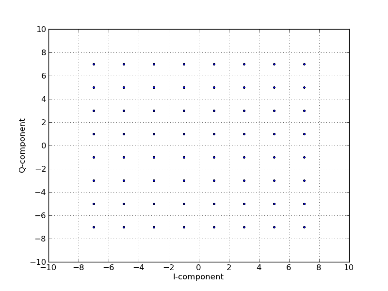
# Ideal 64-QAM constellation
plt.figure(1)
plt.plot(real(tx_sc_symbols), imag(tx_sc_symbols), '.b')
plt.xlabel('I-component')
plt.ylabel('Q-component')
plt.xticks(arange(-10, 12, 2))
plt.yticks(arange(-10, 12, 2))
plt.xlim(-10, 10)
plt.ylim(-10, 10)
plt.grid(True)

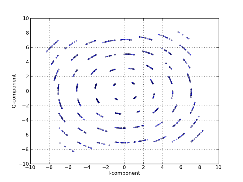
# 64-QAM constellation for Single Carrier with Frequency offset
plt.figure(2)
plt.plot(real(rx_sc_symbols), imag(rx_sc_symbols), '.b', alpha=0.5)
plt.xlabel('I-component')
plt.ylabel('Q-component')
plt.xticks(arange(-10, 12, 2))
plt.yticks(arange(-10, 12, 2))
plt.xlim(-10, 10)
plt.ylim(-10, 10)
plt.grid(True)

# Generate OFDM signal (single symbol) using modulated symbols
tx_ofdm_waveform = ifft(tx_sc_symbols)
# Add frequency offset to the OFDM signal
rx_ofdm_waveform = add_frequency_offset(tx_ofdm_waveform, Fs, delta_f)
# OFDM Demodulation to extract the 64-QAM symbols
rx_ofdm_symbols = fft(rx_ofdm_waveform)

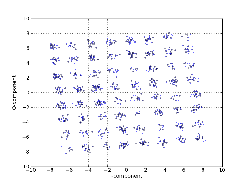
# 64-QAM Constellation for OFDM with Frequency offset
plt.figure(3)
plt.plot(real(rx_ofdm_symbols), imag(rx_ofdm_symbols), '.b', alpha=0.6)
plt.xlabel('I-component')
plt.ylabel('Q-component')
plt.xticks(arange(-10, 12, 2))
plt.yticks(arange(-10, 12, 2))
plt.xlim(-10, 10)
plt.ylim(-10, 10)
plt.grid(True)

plt.show()

We have to look at the received IQ symbols to study the effect of frequency offset. Shown below are the IQ-constellations generated during the simulation.

As seen from the figures above, the constellation points are rotated by varying amounts in the case of a single carrier system whereas, in the case of an OFDM system the constellation points appear noisy. To answer the question of why this difference in the received constellation, we can do a mathematical analysis of the both the systems as follows.

Assumptions and Parameters

Ideal System with frequency offset as the only impairment
Modulation Scheme : 64-QAM
Sampling Frequency ($F_s$) : 15.36 MHz
FFT Size in OFDM : 1024 subcarriers
Number of Bits : 6144 (equivalent to 1024 64-QAM symbols)

Single Carrier System

Let us denote, the 64-QAM modulated IQ symbols at the transmitter by $x(n)$, the 64-QAM modulated IQ symbols at the receiver by $r(n)$, the frequency offset (in Hz) introduced by $\Delta f$, the sampling frequency (in Hz) of the system by $F_s$.

The relationship between $r(n)$ and $x(n)$ is expressed as $$ r(n)=x(n) e^{j2\pi \Delta f n F_s} $$ This can be further modified as $$r(n)=A(n)e^{j\theta(n)}e^{j2\pi \Delta fn F_s}$$ $$r(n)=A(n)e^{j(\theta(n)+j2\pi \Delta f n F_s)}$$ where $A(n)$ and $\theta(n)$ are the magnitude and the phase of the symbol $x(n)$ respectively. From these equations, it is clear that the frequency offset introduces varying amounts of phase offset depending on the time instant n of the modulated symbol $x(n)$. This explains the varying rotation of the received constellation points observed in Figure 2.

OFDM System

Let us denote, the 64-QAM modulated IQ symbols at the transmitter by $X(k)$, the OFDM signal at the transmitter by $x(n)$, the OFDM signal at the receiver by $r(n)$, the 64-QAM modulated IQ symbols at the receiver by $R(k)$, the frequency offset (in Hz) introduced by $\Delta f$,the sampling frequency (in Hz) of the system by $ F_{s}$ , the sub-carrier spacing (in Hz) of the system by $\Delta f_c$, the number of subcarriers (size of the DFT/IDFT) by $N$.

The OFDM signal is generated from the modulated symbols using a inverse Discrete Fourier Transform (IDFT) and is given by

$$ x(n) = \sum_{n=0}^{N-1} X(k)e^{j2\pi k n N} $$

The relationship between $r(n)$ and $x(n)$ is expressed as

$$ r(n) = x(n)e^{j2\pi\Delta f n F_s} $$

From the modulation property of the DFT and noting that $\Delta f_c = \frac{F_s}{N}$, we can express the received 64-QAM modulated symbols as

$$ R(k) = X\bigg(k−\frac{\Delta f}{\Delta f_c}\bigg) $$

Thus the effect of the frequency offset is a change in the sampling instants of the modulated symbols. To express $R(k)$ in terms of $X(k)$, we invoke the Sampling theorem as follows. The continuous time representation $x(t)$ is given by,

$$ x(t) = \sum_{k=-\infty}^{\infty} X(k) \frac{sin(\pi (2Wt−k))}{\pi (2Wt−k)} $$

where $W$ represents the baseband bandwidth of the signal. Therefore, $R(m)$ is given by

$$ R(m) = X\bigg(m−\frac{\Delta f}{\Delta f_c}\bigg) $$

$$ R(m) = \sum_{k=-\infty}^{\infty} X(k)\frac{sin(\pi(\frac{2W}{F_s} (m−\frac{\Delta f}{\Delta f_c})−k))}{\pi(\frac{2W}{F_s} (m−\frac{\Delta f}{\Delta f_c})−k)} $$

Assuming $F_s = 2W$ to simplify the equation we have,

$$ R(m) = \sum_{k=-\infty}^{\infty} X(k)\frac{sin(\pi (m−\frac{\Delta f}{\Delta f_c}−k))}{\pi(m−\frac{\Delta f}{\Delta f_c}−k)} $$

This equation shows us that every received IQ symbol is the sum of scaled versions of all the transmitted IQ symbols, the scaling factor depends on $m$, $k$ and the ratio $\frac{\Delta f}{\Delta f_c}$.

The key point to note is that every IQ symbol (subcarrier) $X(k)$ is a random variable (assuming the data is random) and hence the received IQ symbol $R(m)$ is a sum of random variables which tends to a Gaussian random variable (by the Central Limit Theorem). This explains the observation in Figure 3, where the IQ constellation points appear to be affected by random noise. Since all the subcarriers interfere with the current subcarrier due to the CFO (loss of orthogonality), the effect of CFO on OFDM systems is commonly known by the term Inter-Carrier Interference (ICI).